Schematic cross-section of the spacewire.

1. Launch the SACAMOS SW1 application.
2. From the file menu chose 'Select MOD' to browse to an existing cable model directory or 'Create MOD' to create a new one. Here we have created a new MOD directory called 'MOD_WEB_EXAMPLES'. Note: that all MOD directories have to reside in the root of the SACAMOS folder.
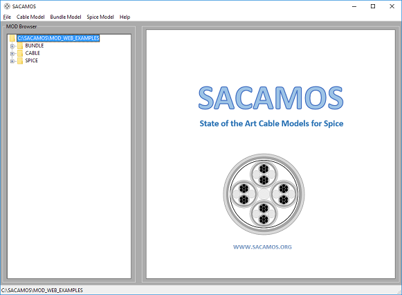
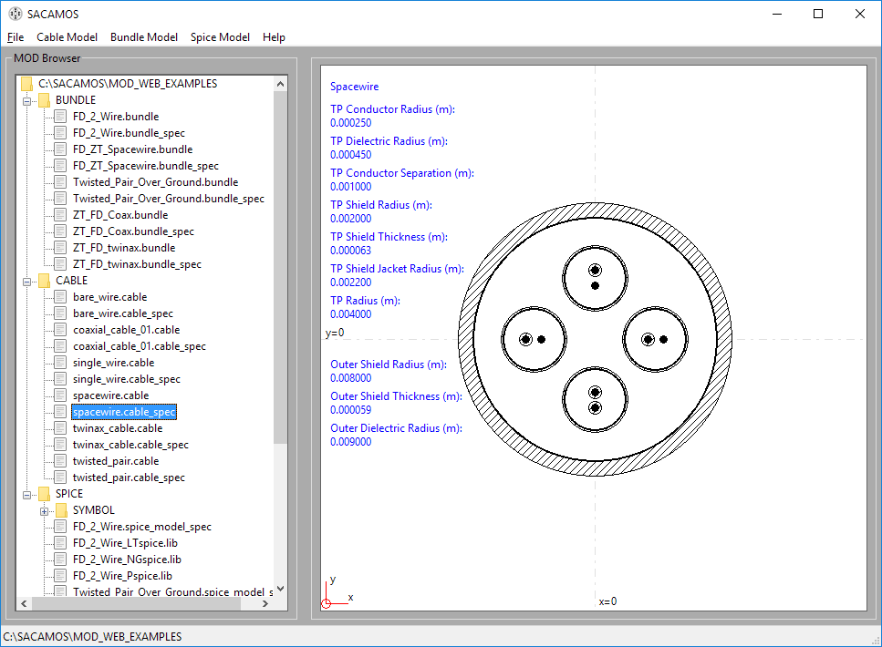
3. Once MOD has been selected the main GUI window will look like:
4. The other menus on the toolbar will now be enabled.

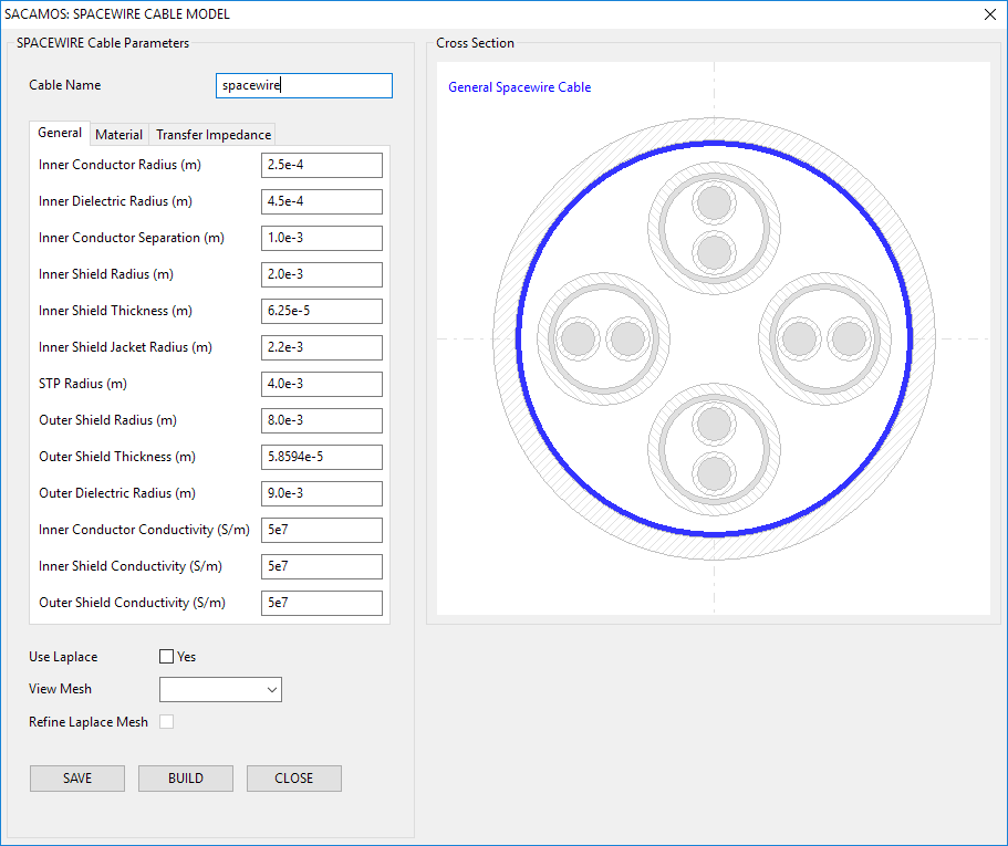
1. From the 'Cable Model' menu chose 'Spacewire'.
2. Enter a name for the cable model e.g. spacewire
3. Now enter the parameters for the cable model, note all dimensions are in meters (m) and can be in floating point or scientific (E) notation :
inner conductor radius = 2.5e-4
inner dielectric radius = 4.5e-4
inner conductor separation = 1.0e-3
inner shield radius = 2.0e-3
inner shield thickness = 6.25e-5
inner shield jacket radius = 2.2e-3 
shielded twisted pair radius = 4.0e-3 
outer shield radius = 8.0e-3
outer shield thickness = 5.8594e-5
outer dielectric radius = 9.0e-3 
inner conductor electric conductivity = 5e7 
inner shield electric conductivity = 5e7 
inner shield electric conductivity = 5e7
.

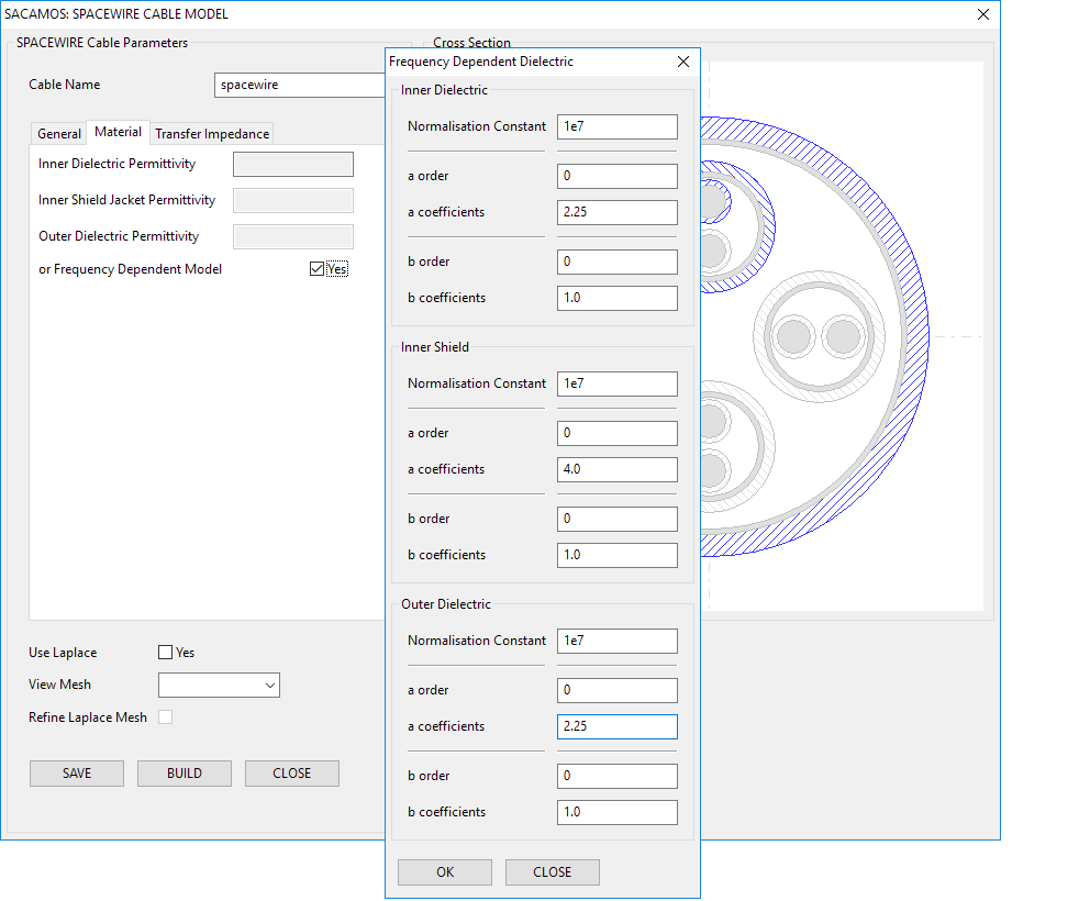
4. To enter the frequency dependent parameters, select 'material' tab and 'tick' the check box and a pop-up window will appear. Enter the following parameters:
Inner dielectric permittivity model:
normalisation constant = 1e7
a order = 0 
a constants = 2.25 
b order = 0 
b constants = 1.0
Inner Shield permittivity model:
normalisation constant = 1e7
a order = 0
a constants = 2.40 
b order = 0
b constants = 1.0
Outer dielectric permittivity model:
normalisation constant = 1e7
a order = 0 
a constants = 2.25 
b order = 0
b constants = 1.0

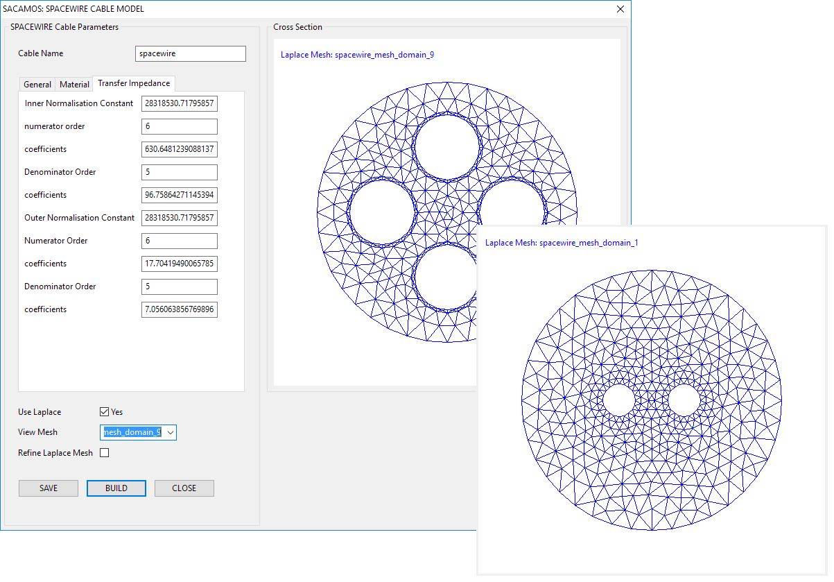
5. Select the 'transfer impedance' tab to define the transfer impedance:
inner normalisation constant = 628318530.71795857
order of numerator model = 6
numerator coefficients = 2.5468494337902981E-002 8.2338738578784980 195.63548903976618 1209.1421442346702
3006.6530418447878 3357.6215437592941 
1630.6481239088137 (Note: this is entered as a space seperated list)

order of denominator model = 5
denominator coefficients = 1.0 23.599449123864371 145.90222072648291 362.78999275303835 405.14016972907552 196.75864271145394 

outer normalisation constant = 628318530.71795857 
order of numerator model = 6
numerator coefficients = 6.7910018908980910E-003 6.3516651586671768 131.85223712596317 714.73088207712362 1550.1604988129416 1509.1499548754166 617.70419490065785
order of denominator = 5
denominator coefficients = 1.0000000000000000 20.715352684308218 112.30217945904732 243.56691527043952 237.12345747204483 97.056063856769896

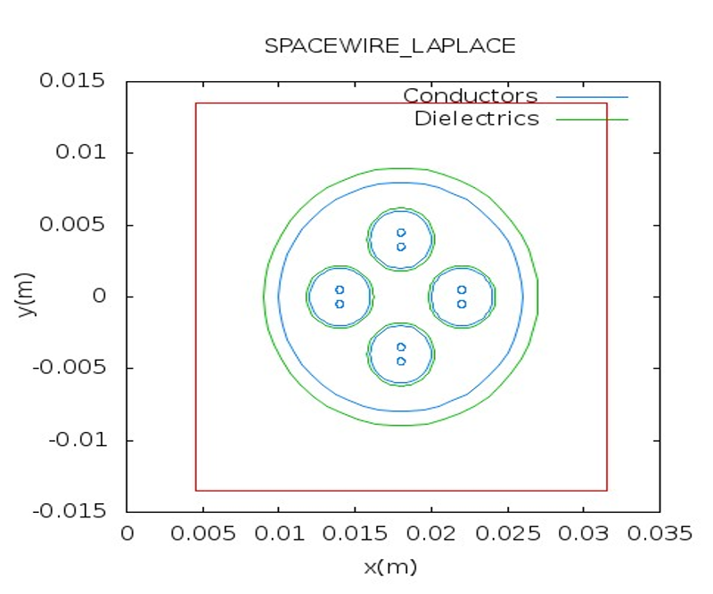
6. This model uses the Laplace solver, therefore tick the box 'Use Laplace'. Click 'SAVE'. If all is correct, the save button will be disabled. Then click 'BUILD'. A terminal window will then appear as the Laplace solver performs the calculations.

Following the build two meshes are viewable, one for the twisted pair cable domain and another for the overall spacewire domain.

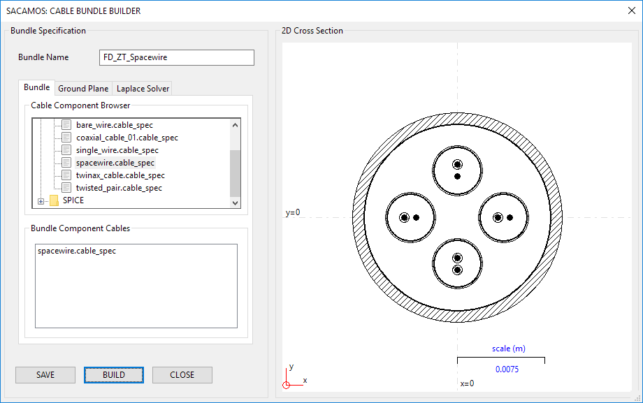
Even though a spice model is required for just a single cable it must first be created as a bundle. Therefore:
1. From the 'Bundle Model' menu chose 'Create Bundle'.
2. Enter a name for the cable bundle model e.g. FD_ZT_Spacewire.
3. Expand the 'Cable' directory on the 'Cable Component Browser'.
4. Double click the 'spacewire' cable in the component browser and enter the required x and y coordinates of the cable's centre (and rotation if appropriate) and click 'OK' to place the cable. Place the cable in the centre of the cross section i.e. x = 0.0, y = 0.0 and rotation = 0.0.
5. Click 'SAVE'. If all is correct, the save button will be disabled. Then click 'BUILD'.
6. The Run Status will appear and state that the cable model builder finished correctly.
7. Close the cable model window.

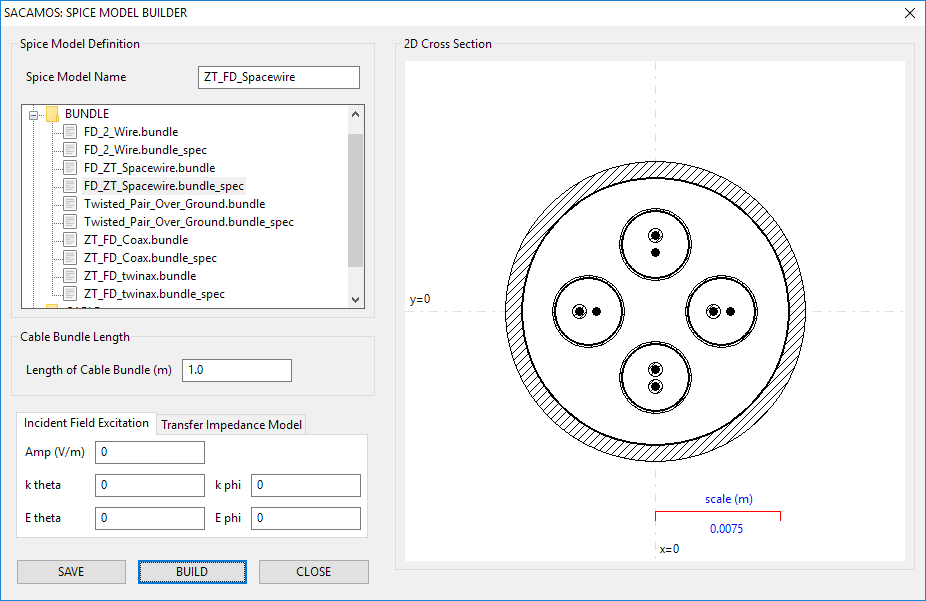
1. From the 'Spice Model' menu chose 'Create Spice Model'.
2. Enter a name for the Spice model e.g. FD_ZT_Spacewire.
3. Expand the 'Bundle' directory in the file browser and select the bundle for which the Spice model is required by double clicking on the '.bundle_spec' file. The schematic will then be displayed.
4. Enter the lenght of cable that the model will represent, in meters, e.g. 1.0.
5. No more details are required for this model. Therefore click 'SAVE' and then 'BUILD'.
6. The Run Status will appear and state that the Spice model builder finished correctly.
7. Close the cable model window.

1. From the main SACAMOS GUI. Expand the 'Cable' and 'Bundle' branches of the 'MOD Browser'. There should be entries for the cable and bundle models created above.
2. Double clicking the 'cable_spec' entries will display the cable or bundle. For cables the relevant data will also be displayed.

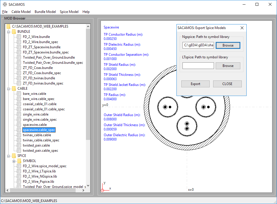
Spice models have now been created for Ngspice, LTspice and Pspice, along with symbols for Ngspice and LTspice. These symbols now need to be placed in the symbol folders for the schematic capture being used. For the example that follows this will be gschem, part of the gEDA suite which requires the '.sym' file.
Note only the symbol files need to be exported the associated ',lib' files remain in the MOD folder and must not be moved as the locationof the .lib file is encoded in the .sym file.
1. From the 'Spice Model' menu chose 'Export Spice Model'.
2. From here browse to the symbol folders for the schematic capture system you are using. For example for gschem installed in the root directory of a Windows system the path is: 'C:\gEDA\gEDA\share\gEDA\sym\local'
3. Click 'EXPORT'
4.Click 'CLOSE'. The symbols can now be used in the schematic capture process...